Introduction to Causality
“Data are profoundly dumb [...].
That’s all a deep-learning program can do : fit a function to data.“
-- Judea Pearl in ”The Book Of Why”
Causality is definitely one of the hottest topic of the recent years, and rightly so ! It is seen as one of the keys to help current AI system reaching a next step towards true intelligence, as highlighted by Turing-Award winner Yoshua Bengio at Neurips 2020 : “[We] won’t deliver a true AI revolution, until it can go beyond pattern recognition and learn more about cause and effect“.
Let’s look at two examples to illustrate why we need causality : (1) an interesting statistical paradox to raise curiosity and (2) the famous brain-teaser Monty Hall problem.
Simpson’s Paradox

Context : we want to investigate which of two treatments on tumor is the most effective. To do so, we come accross a study that have been conducted over the years, aiming at comparing the recovery rate between our two treatments of interest : A (Take medication) and B (Have surgery). At first sight, the data collected seems to be quite decent : around 2000 patients (quite as sample!) have been given either treatment A or B in equal proportion.
Question : If tomorrow I’m diagnosed a tumor, which one of the two treaments should I take ?
First instinct would be to simply look at the global recovery rate of the two subgroups, the ones who have been given treatment A (medication) against the ones who have received treatment B (surgery).
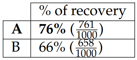
Anyone after looking at the data would have this gut feeling that treatment A seems to be better suited to recover from a tumor. Let’s bring the medication ! .. well not so fast !!
The “size of the tumor” feature have been collected in the data, sorting tumor in two subgroups “small” or “big” based on the diameter of the tumor. Let’s have a look a it :
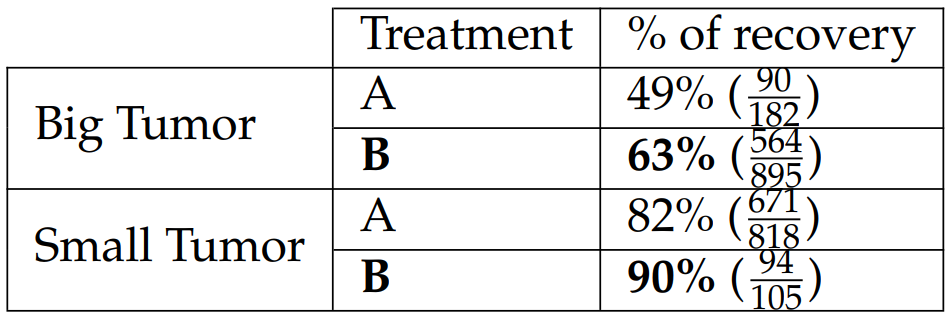
Treatment B, i.e having surgery, seems to be better for small tumors .. and better as well for big tumors. How come Treatment B now be better for both groups ? Figures from both tables come from the same survey but now leads to two really distinct conclusions !
Historically, as a matter of life/death decisions when dealing with big tumors, patients would most of the time be given surgery. By nature, bigger tumors leads to a lower recovery rate (due to higher risks of complications) and to a more recurrent use of surgery. The size of the tumor acts here as a confounding factor.
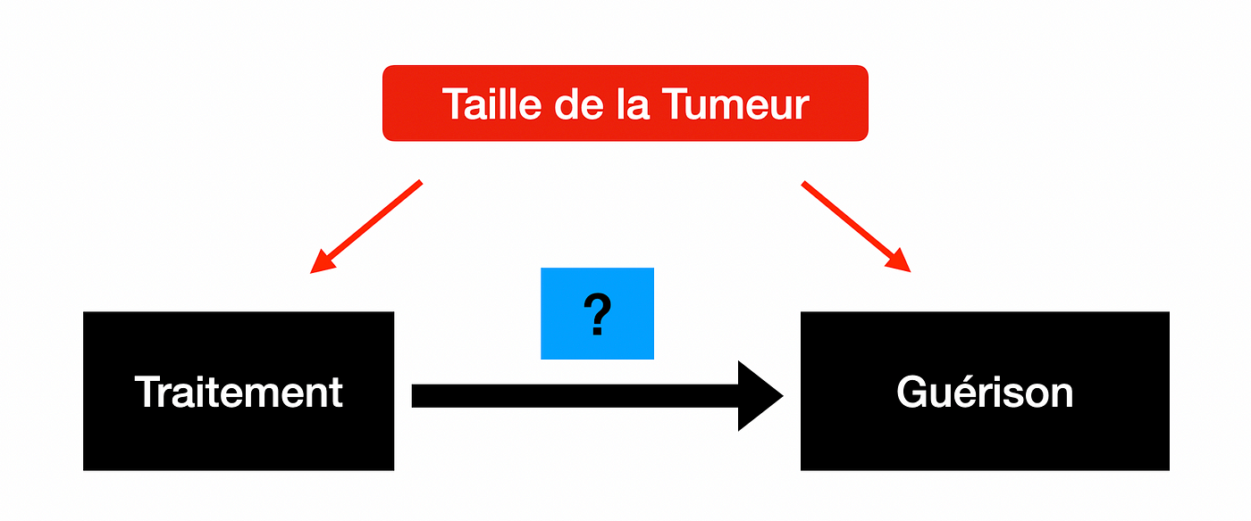
We are studying the causal effect between X(treament) → Y (recovery), but a third variable Z which is the size of the tumor affects both the recovery and the treatment given in our observational dataset. One has to be careful when using retrospective studies - in contrast with projective study where links between potential confounding factors and causes can be broken with randomization for instance.
Monty Hall Problem
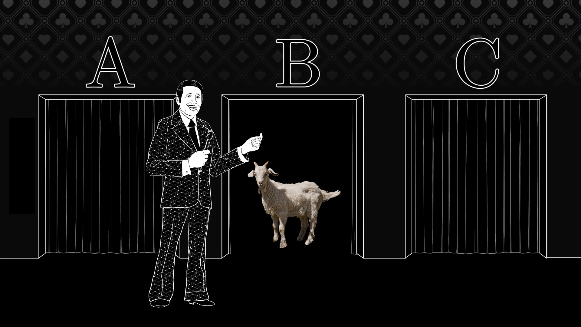
This problem is named after Monty Hall, who hosted the tv game show Let’s Make a Deal between the 60s and the 80s.
The game setting is pretty simple : you’re given the choice of three doors, behind one of them is a Cadillac, behind the others two, goats. If you open the right door, you go home in a brand new car, otherwise you go home with a goat.
- Your start by picking a door, with a probability 1/3 of winning the car.
- Instead of opening the door you picked, Monty, who by the way knows what's behind each doors, opens one of the two other doors. Big suprise, here is a goat.
- Then, Monty says to you "Do you want to keep your original pick or do you want to switch doors ?"
Question : Is it to your advantage to change your choice?
The naive way to solve this would be to think that I have now a choice between two doors with both probability 1/2 to hide the car. Why bother changing my choice if both doors has the same probability ?
Let’s change slighlty the perspective here. By using the Bayes formula, the probability that the car remains behind our initial pick, knowing that a goat was behind the door open by Monty, stays the same as before : P(Door picked | Second Door opened) = 1/3. On the contrary, the conditional probability of the third door of hidding the car becomes now P(Third Door | Second Door open ) = 2/3. Following this intuition, we better change our choice to the third door !
Mathematician Marilyn vos Savant, who proposed this solution when asked in “Ask Marilyn” column in Parade magazine in 1990, got hugely criticized for it, even by other prestigious mathematicians of the time.
One way to prove this is to experimentally and numerically compute the mean reward R obtained in this problem. This indeed leads to a mean reward of 2/3 when switching doors, and 1/3 by keeping the first pick. Another way to understand what happens here is to use Causality !
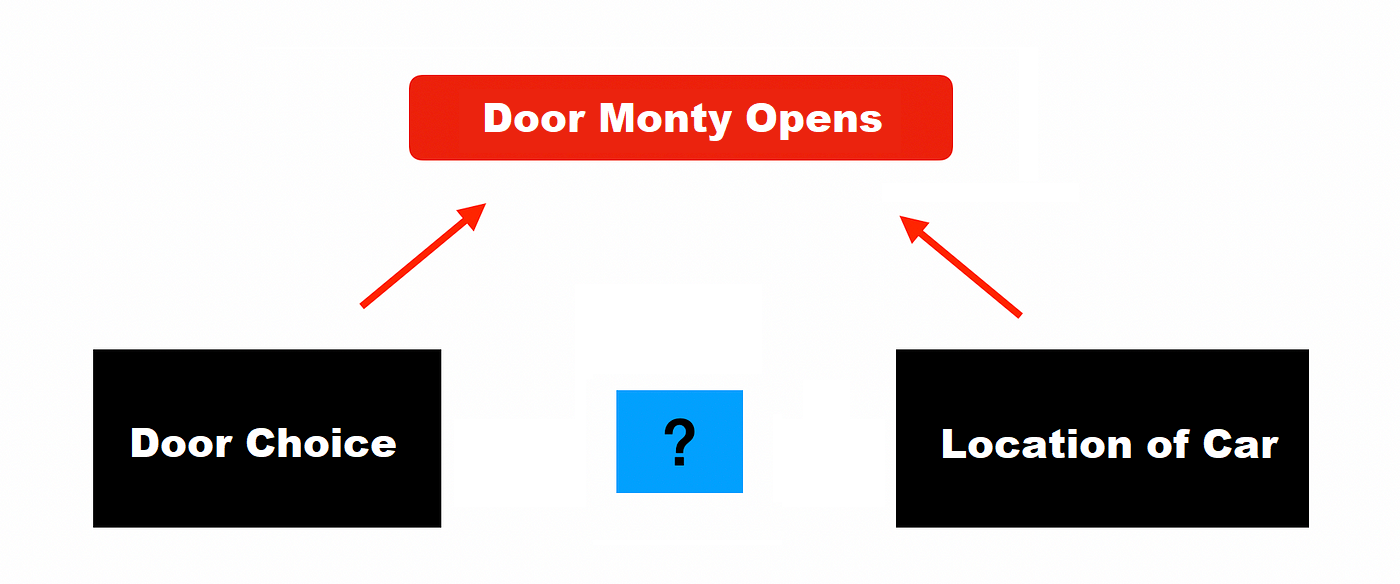
Notice how different the arrow in the diagram are from the Simpson’s Paradox one. When we were dealing with a confounder earlier, i.e a third variable that affects both the input and output, we now are in presence of a collider.
For clarity, let’s have A=”Door Choice”, B=”Car’s location”, C=”Door opened by Monty”. Here, our intuition should tell us that A and B looks independant (and they are). Our choice of picking one of the three doors doesn’t change the car’s location (and vice-versa). On the other hand, A and C are dependant as Monty adapts which door he opens regarding our initial pick. Same with B and C as Monty makes sure he only reveals a goat and not the car.
That’s where it comes interesting : when we condition on C (we “fix” C, which becomes the case as Monty opens a door and reveals a goat.), causality tells us it creates a spurious association between the other two variables A and B. As a result, A and B become dependant variables. Conclusion, if intuition tells you at first that the door you pick and the door the car is behind are independent, the information brought when Monty opens a door (based on both your choice AND the car’s location), THEN your choice of a door and the car’s location becomes spuriously associated by Monty Hall’s control of which door he opens.
Do-Calculus and Pearl’s Framework
“Statistics focused exclusively on how to summarize data, not on how to interpret it [...]. Data can tell you that people who took a medicine recovered faster than those who did not, but they can’t tell you why.“
-- Judea Pearl in ”The Book Of Why”
Judea Pearl introduced the concept of Ladder of Causation, as a conceptual and abstract way to sort the different levels at which us, as human, reason. It captures the differents and gradual notions of causality, and accounts for the next challenges machine learning will have to face :
- Association - the first level consists in seeing, or observing, which cover most of the robot and animal's learning. It enables to answer questions like "What if I see ..?", "How are the variables related" or "How would seeing X change my belief in Y"? It corresponds to the estimation of .
- Intervention - the next level enables you to act within your environment and witness the results of your own actions. It allows you to answer question like "What if I do ..?", "How can I make .. happen?" or "What would Y become if I do X"?. It is really crucial to grasp the difference between the first and second level because here is introduced the notion of causality between what I see and what I do. We aim at estimating .
- Counterfactual - the last, but no least, level of the ladder introduces imagination. What makes human reasoning so singular is its ability to reason counterfactually, that is to say, answer to question like "What if i acted differenty?" or "Why did it happen?". This retrospection enables humans to get a much better understanding of their environment and increases significantly their capacity to learn, and to learn quickly.
The ladder of Causation with an Example
Level 1 - Association What does a symptom tell me about a disease ?
Level 2 - Intervention What if I take an aspirin, will my headache be cured ?
Level 1 - Counterfactual
Was it my aspirin that stopped my headache?
What woud have happen if I took something else ?
Do-Calculus
So as to fill the gap between the first two levels, Pearls introduced the framework of do-calculus. It plays a major role in relating both observational distributions p(Y|X) and interventional distributions p(Y|do(X)). Basically, we are interested in measuring changes in distribution of some random variables {X, Y, Z, ..} when one performs an intervention do(x), which forces the random variable X to take the value x, regardless of its causes (or causal ancestors). To do so, one uses a set of rules which allows for measuring and indentifying interventional queries, when specific structural conditions are met in the causal DAG (directed acyclic graph). The main goal is to make interventional queries identifiable, i.e that can be expressed in terms of observational distributions, without the do operator.
Consider a set of random variables {X, Y, Z, W} along with their associated DAG G :
- Rule 1 - Insertion/delation of observations : if Y and Z are d-separated by in - from G by removing arrows pointing into X -, then :
- Rule 2 - Exchange action/observation : if Y and Z are d-separated by in G+- from G by removing arrows pointing into X and arrows pointing out of Z-, then :
- Rule 3 - Insertion/Delation of actions : if Y and Z are d-separated by in G++ - from G by (1) removing arrows pointing into X (G*) then (2) removing arrows pointing to Z that are not ancestors of any variable W in G*-, then :